Unsupervised learning
Self-supervised Visual Feature Learning with Deep Neural Networks: A Survey,PAMI20
A Survey on Semi-, Self- and Unsupervised Learning in Image Classification,Arxiv2002
check zhihu discussion
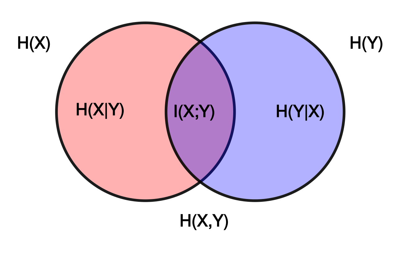
Mutual Information
I(X;Y)=0 if X and Y is unrelated. otherwise I(X;Y) is larger than zero.
Intuitively, mutual information measures the information that X and Y share: It measures how much knowing one of these variables reduces uncertainty about the other. If X=Y+3 or X=Y^3, which means X is a deterministic function of Y and vice versa, then mutual information I(X;Y) is the entropy of Y(or X).
Property: Non-negativity, and Symmetry.
TO CONTINUE
Normalized Mutual Information (NMI):
\[NMI(A;B) = \frac{I(A;B)}{\sqrt{H(A)H(B)}}\]LeCun’s opinion between self-supervised learning and unsupervised learning
https://www.facebook.com/yann.lecun/posts/10155934004262143
Visual Task Adaptation Benchmark
Similarly, representations may be pre-trained on any data, VTAB permits supervised, unsupervised, or other pre-training strategy. There is one constraint: the evaluation datasets must not be used during pre-training. This constraint is designed to mitigate overfitting to the evaluation tasks.
A broadly used method in NLP, also used in CPC: Representation Learning with Contrastive Predictive Coding,Arxiv18, Unsupervised Feature Learning via Non-Parametric Instance Discrimination,CVPR18, etc.
Originally proposed in 2010, used in NLP from this paper: A fast and simple algorithm for training neural probabilistic language models. In NLP, NCE fixes the value of normalizer Z, making the inference (if you need probability values) faster. You don’t need to sum over all the vocabulary to get the normalizer value.
The reason why NCE loss will work is because NCE approximates maximum likelihood estimation (MLE) when the ratio of noise to real data 𝑘 increases.
Negative Sample is a special case of NCE, for reason you can check the summary of approximating softmax, also you can check a detailed comparison between negative sample and NCE in this note: Notes on Noise Contrastive Estimation and Negative Sampling
A fast and simple algorithm for training neural probabilistic language models
Motivation of this work is based on the following points:
- gradient-based back propogation is a must.
- We cannot sum over all vocabulary to get the normalizer value, then we need to approximate it.
- Why not approximate it from the perspective of gradient?
- softmax classifier summarize the classification problem as a N-class problem, NCE summarizes the classification problem as a binary-class problem. Even though, the gradient derivation pattern is similar.
Equation 10 can be derived by normal derivation rule.
Equation 11 is from the definition of expectation.
TODO, why Equation 12 is the Maximum Likelihood gradient
Unsupervised Feature Learning via Non-Parametric Instance Discrimination,CVPR18
maintain a image-levell memory bank. Check Fig 2.
use noise-contrastive estimation[NCE]
The conceptual change from class weight vector wj to feature representation vj directly is significant. The weight vectors {wj} in the original softmax formulation are only valid for training classes. Consequently, they are not generalized to new classes, or in our setting, new instances. When we get rid of these weight vectors, our learning objective focuses entirely on the feature representation and its induced metric, which can be applied everywhere in the space and to any new instances at the test.
Computing the non-parametric softmax above is cost prohibitive when the number of classes n(n images in the dataset) is very large, e.g. at the scale of millions. The solution is to cast the multi(n)-class classification problem into a set of binary classification problems, where the binary classification task is to discriminate between data samples and noise samples.
K-pair Loss: Improved Deep Metric Learning with Multi-class N-pair Loss Objective,NIPS16
Contrastive Representation Distillation,ICLR20
Drop-in replacement for Knowledge Distillation, with state of the art performance
Mutual Information Gradient Estimation for Representation Learning,ICLR20
CMC: Contrastive Multiview Coding
an extension based on CPC.
check session 2.2
CPC: Representation Learning with Contrastive Predictive Coding,Arxiv18
The key insight of CPC is to learn such representations by predicting the future in latent space by using powerful autoregressive models.
Check NIPS invited talks here
For a brief summary, you can check the session 2 of this paper.
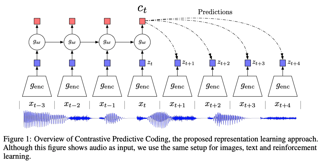
Basic idea
latent representations \(z_{t}=g_{enc}(x_{t})\). An autoregressive model \(g_{ar}\) summarizes all z<=t in the latent space and produces a context latent representation \(c_{t}=g_{ar}(z\le t)\).
Mutual information between original signal x and c: \(I(x;c) = \sum_{x,c} p(x,c) log \frac{p(x|c)}{p(x)}\), here is another writing of mutual information because of the bayesian rule(common rule, no extra condition is needed).
predict future observations as \(\frac{p(x_{t+k}|c_{t})}{p(x_{t+k})}\) rather than \(p_{k}(x_{t+k}|c_{t})\)
In reality, a simple log-bilinear model \(f_{k}(x_{t+k},c_{t})=exp(z^{T}_{t+k}W_{k}c_{t})\) is used. The authors precise that the linear transformation \(Wc_{t}\) can be replaced by non-linear models like neural nets.
Given X=\(x_{1},...,x_{N}\) of N random samples containing one positive sample from \(p(x_{t+k}|c_{t})\) and N-1 negative samples from the ‘proposal’ distribution \(p(x_{t+k})\) The final loss(InfoNCE loss) is:\(\mathcal{L}_{N} = - \mathbb{E}_{X} [ log \frac{f_{k}(x_{t+k},c_{t})}{\sum_{x_{j} \in X} f_{k}(x_{j},c_{t})}]\)
Considering \(f_{k}(.,.)\) is a log-bilinear model, InfoNCE loss can also be viewed as a softmax loss.
Optimizing InfoNCE loss is optimizing a lower bound on the mutual information between x and c.
The observation(game rule) is 1 positive sample from \(p(x_{t+k}/c_{t})\) and N-1 negative samples from \(p(x_{t+k})\). Each event contains 1 positive sample and N-1 negative samples, that’s the rule defining an event.
Therefore, The probability of that the i-th sample is positive(meantime the other N-1 is negative) is:
\[p(d=i|X,c_{t}) = \frac{p(x_{i}|c_{t})\prod_{l \neq i} p(x_{l})}{\sum_{j=1}^{N} p(x_{j}|c_{t}) \prod_{l \neq j} p(x_{l})} = \frac{p(x_{i}|c_{t})/p(x_{i})}{\sum_{j=1}^{N} p(x_{j}|c_{t})/p(x_{j})}\]A futher provement relating InfoNCE and \(p(d=i|X,c_{t})\) can be seen in supplimentary file.
TODO, cannot figure out the logic from Equation 10 to Equation 11. how to induce p(x,c) is equivalant to p(x)?
After finishing traing by InfoNCE loss, the \(g_{enc}\) is trained optimally so that it can be utilized in many downstream tasks.
CPCv2: Data-Efficient Image Recognition with Contrastive Predictive Coding
DIM: Learning deep representations by mutual information estimation and maximization,ICLR19,oral
AMDIM:Learning Representations by Maximizing Mutual Information Across Views
self-supervised representation learning based on maximizing mutual information between features extracted from multiple views(multiple augmentations) of a shared context(same image)
based on previous work Deep InfoMax(DIM,2019).Our model, which we call Augmented Multiscale DIM (AMDIM), extends the local version of Deep InfoMax introduced by Hjelm et al. [2019] in several ways. First, we maximize mutual information between features extracted from independently-augmented copies of each image, rather than between features extracted from a single, unaugmented copy of each image.2 Second, we maximize mutual information between multiple feature scales simultaneously, rather than between a single global and local scale. Third, we use a more powerful encoder architecture. Finally, we introduce mixture-based representations. We now describe local DIM and the components added by our new model.
TODO
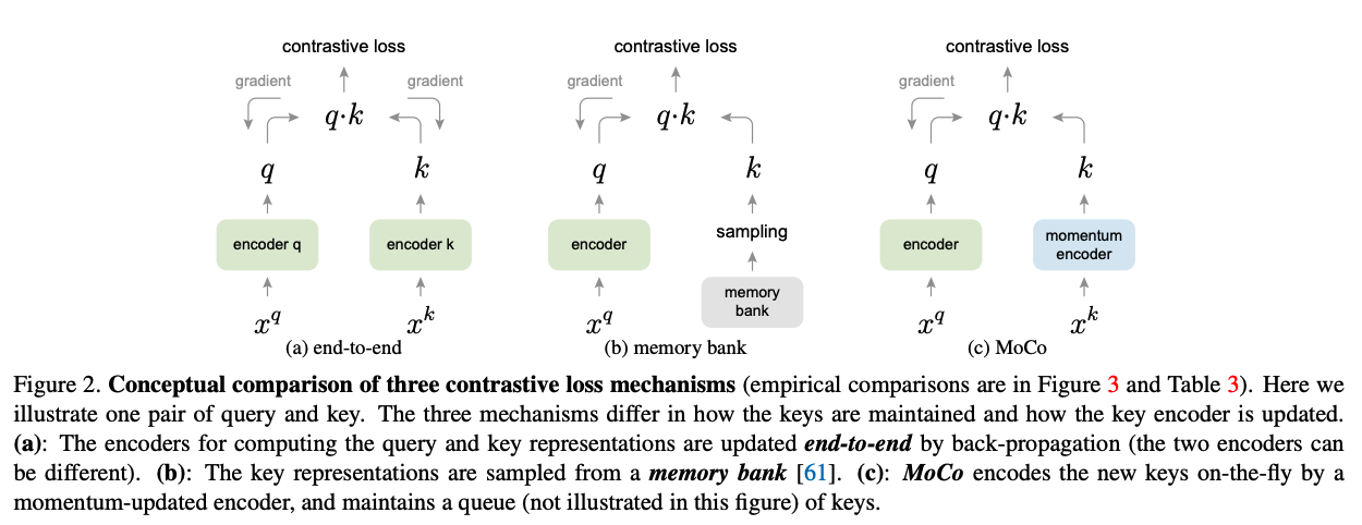
MoCo: Momentum Contrast for Unsupervised Visual Representation Learning,CVPR20
Preliminary: InfoNCE paper.
A contrastive loss function, called InfoNCE, is considered in this paper. Contrastive loss functions can also be based on other forms , such as margin-based losses and variants of NCE losses. Difference between infoNCE: 1) W in C_{t}W x is inogred here by directly dot product.
labels = zeros(N): nn.CrossEntropyLoss((N),Nx(K+1)), positive sample is always first, therefore labels is all zero.
Relationship with previous works: Compared to another similar idea of memory bank (Wu et al, 2018) which stores representations of all the data points in the database and samples a random set of keys as negative examples, a queue-based dictionary in MoCo enables us to reuse representations of immediate preceding mini-batches of data.
Motivation of queue setting: removing the oldest mini-batch can be beneficial, because its encoded keys are the most outdated and thus the least consistent with the newest ones.
Motivation of moment update: Using a queue can make the dictionary large, but it also makes it intractable to update the key encoder by back-propagation (the gradient should propagate to all samples in the queue).
dictionary size can be much larger than a typical mini-batch size, and can be flexibly and independently set as a hyper-parameter.
momentum update is on the parameter of the encoder, not the feature of samples. same pattern also occurs in mean teacher paper.
In experiments, a relatively large momentum (e.g., m = 0.999, our default) works much better than a smaller value (e.g., m = 0.9), suggesting that a slowly evolving key encoder is a core to making use of a queue. The temperature in InfoNCE in is set as 0.07. We set query length K = 65536.
In experiments, we found that using BN prevents the model from learning good representations, as similarly reported in [35] (which avoids using BN). The model appears to “cheat” the pretext task and easily finds a low-loss solution. This is possibly because the intra-batch communication among samples (caused by BN) leaks information. check A.9. Ablation on Shuffling BN
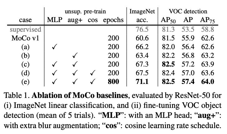
MoCo V1’s focus is on a mechanism for general contrastive learning; we do not explore orthogonal factors (such as specific pretext tasks) that may further improve accuracy. As an example, “MoCo v2”, an extension of a preliminary version of this manuscript, achieves 71.1% accuracy with R50 (up from 60.6%), given small changes on the data augmentation and output projection head. We believe that this additional result shows the generality and robustness of the MoCo framework.
MoCo v1/2 is also useful in CURL which finds MoCo “is extremely useful in Deep RL” (quote Aravind Srinivas, CURL author).<CURL: Contrastive Unsupervised Representations for Reinforcement Learning>
Happen to see this nice video introducing MoCo v1/v2! It also covers Berkeley's recent work on CURL which finds MoCo "is extremely useful in Deep RL" (quote Aravind Srinivas, CURL author).
Posted by Kaiming He on Wednesday, April 15, 2020
Negative Margin Matters: Understanding Margin in Few-shot Classification,Arxiv2003
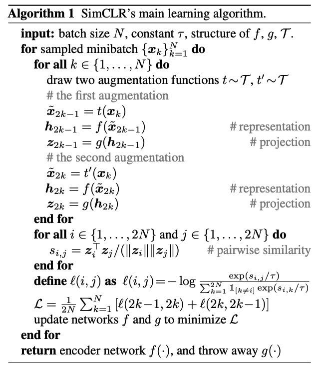
SimCLR:A Simple Framework for Contrastive Learning of Visual Representations
from Mocov2:
SimCLR [2] improves the end-to-end variant of instance discrimination in three aspects: (i) a substantially larger batch (4k or 8k) that can provide more negative samples; (ii) replacing the output fc projection head [16] with an MLP head; (iii) stronger data augmentation.
check zhihu
- about cosine similarity: https://github.com/google-research/simclr/issues/38
- With 128 TPU v3 cores, it takes ∼1.5 hours to train our ResNet-50 with a batch size of 4096 for 100 epochs.
- the combination of random crop and color distortion is crucial to achieve a good performance
- check supplimentary, find a detailed comparison with previous methods.
SimCLR2: Big Self-Supervised Models are Strong Semi-Supervised Learners
- 128 Cloud TPUs, with a batch size of 4096.
- The proposed semi-supervised learning algorithm can be summarized in three steps: unsupervised pretraining of a big ResNet model using SimCLRv2 (a modification of SimCLR [1]), supervised fine-tuning on a few labeled examples, and distillation with unlabeled examples for refining and transferring the task-specific knowledge.
Spatiotemporal Contrastive Video Representation Learning,Arxiv2008
simclr in video, compare with inflated simclr…
Unsupervised Learning by Predicting Noise
On Mutual Information in Contrastive Learning for Visual Representations,Arxiv2005
On Mutual Information Maximization for Representation Learning,ICLR20
check concolusions.
it is unclear whether the connection to MI is a sufficient (or necessary) component for designing powerful unsupervised representation learning algorithms. We propose that the success of these recent methods could be explained through the view of triplet-based metric learning and that leveraging advances in that domain might lead to further improvements.
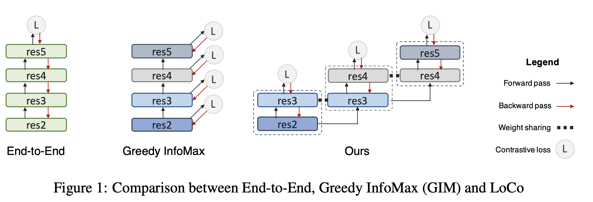
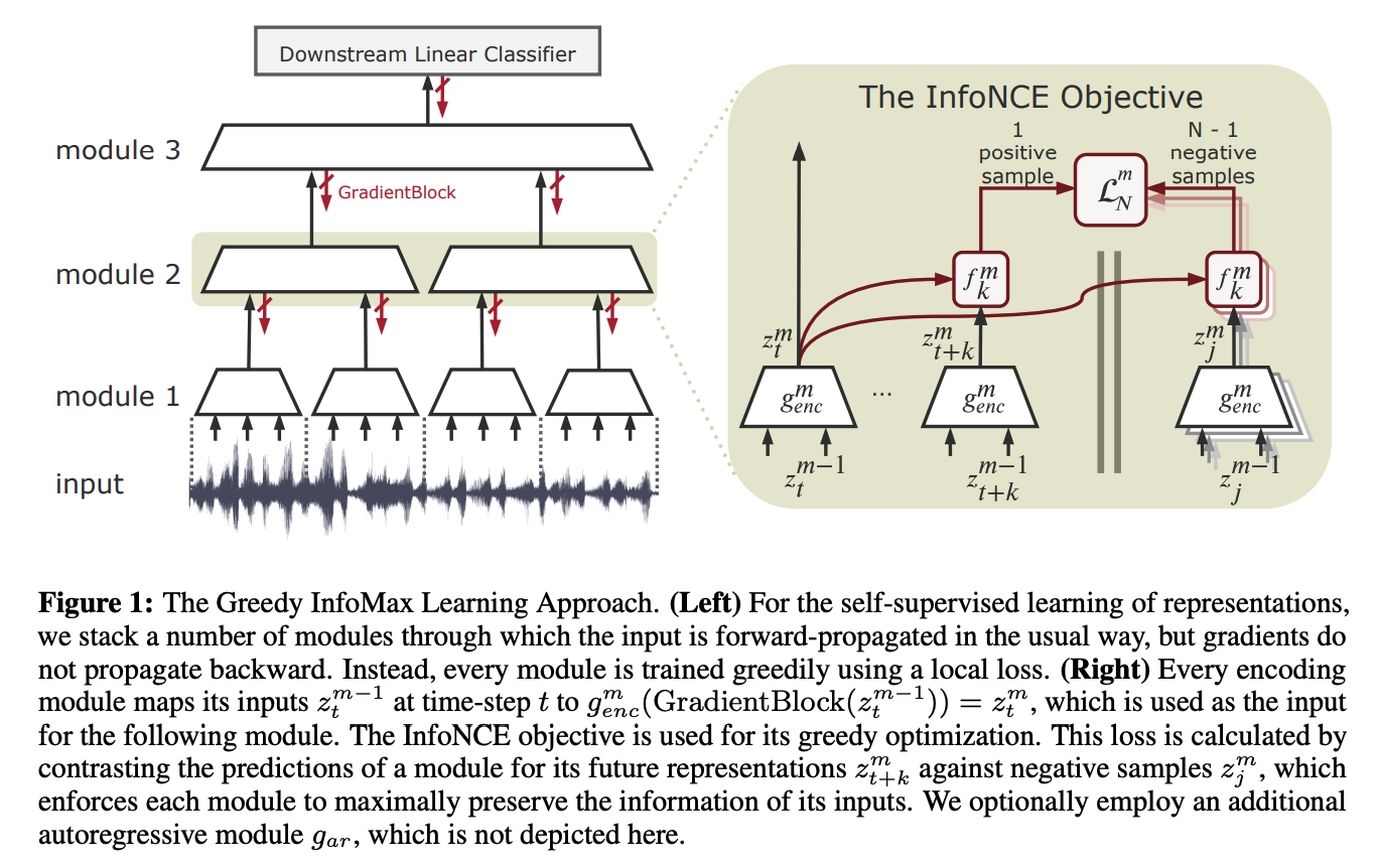
Greedy InfoMax:Putting An End to End-to-End:Gradient-Isolated Learning of Representations,NIPS19
without end-to-end backpropagation != without backpropagation
multiple-losses(multiple optimizers) backward
Gradient is isolated between modules, but still need gradient in modules. Each module will generate a CPC loss.
For vision task context feature c is replaced by z for simplicity.
LoCo: Local Contrastive Representation Learning,Arxiv2008
Extension on greedy infomax
How Useful is Self-Supervised Pretraining for Visual Tasks? see observation from CVPR20
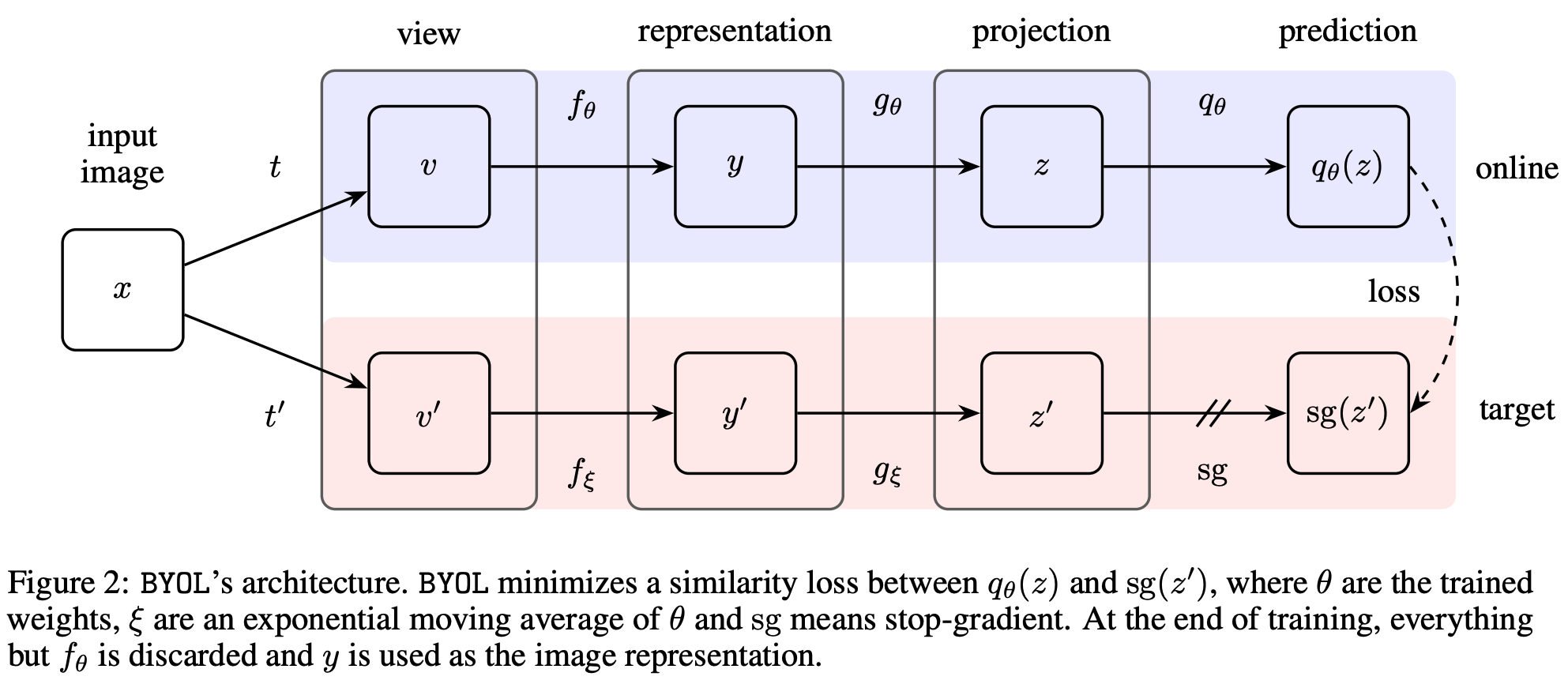
BYOL:Bootstrap Your Own Latent A New Approach to Self-Supervised Learning,NeurIPS20
without using negative pair This experimental finding is the core motivation for BYOL: from a given representation, referred to as target, we can train a new, potentially enhanced representation, referred to as online, by predicting the target representation. From there, we can expect to build a sequence of representations of increasing quality by iterating this procedure, using subsequent online networks as new target networks for further training.
- result is worse than Contrasting Cluster Assignments.
PCL: Prototypical Contrastive Learning of Unsupervised Representations,Arxiv2005
result is worse than https://arxiv.org/pdf/2006.09882.pdf
A critical analysis of self-supervision, or what we can learn from a single image,ICLR20
We evaluate self-supervised feature learning methods and find that with sufficient data augmentation early layers can be learned using just one image. This is informative about self-supervision and the role of augmentations.
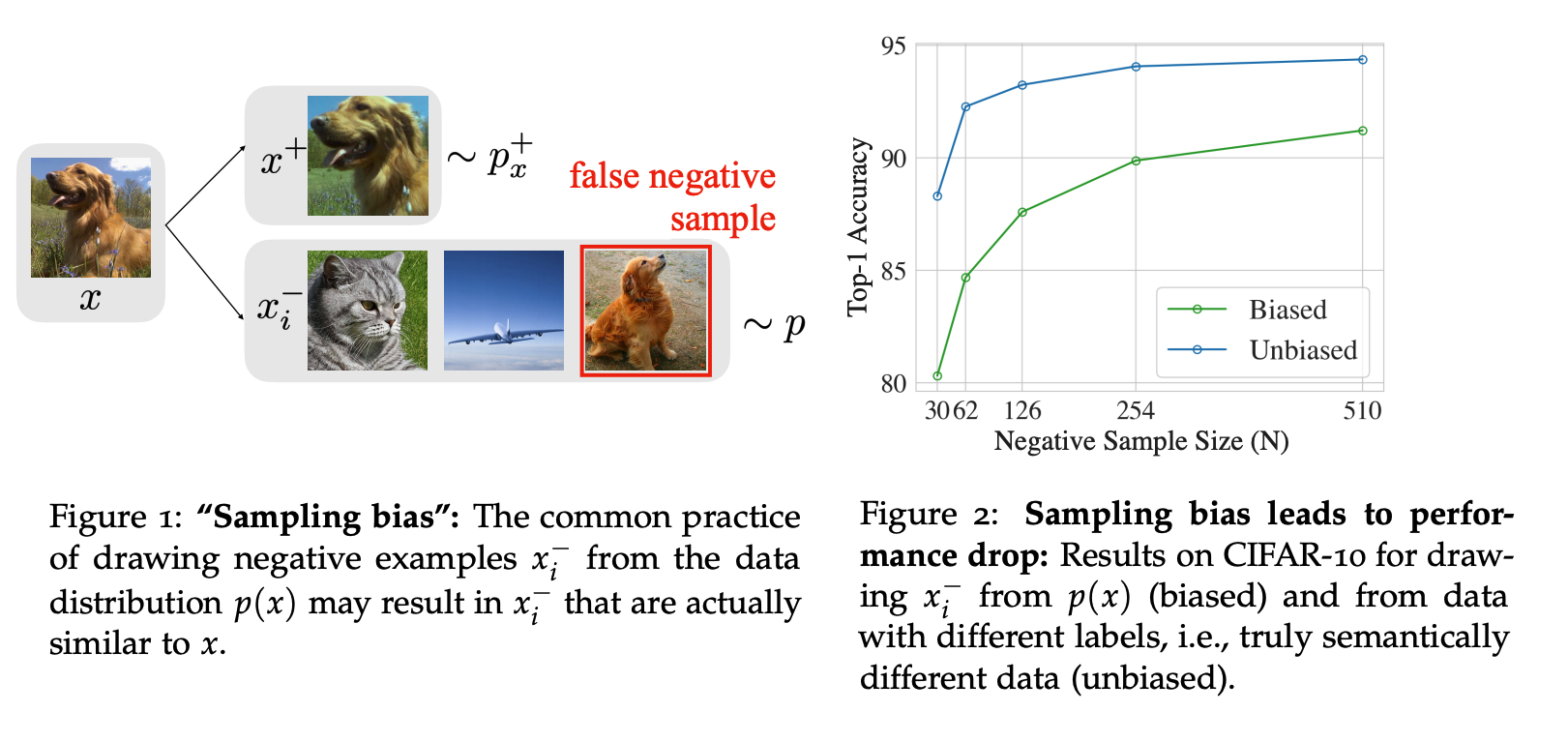
Debiased Contrastive Learning,Arxiv2007
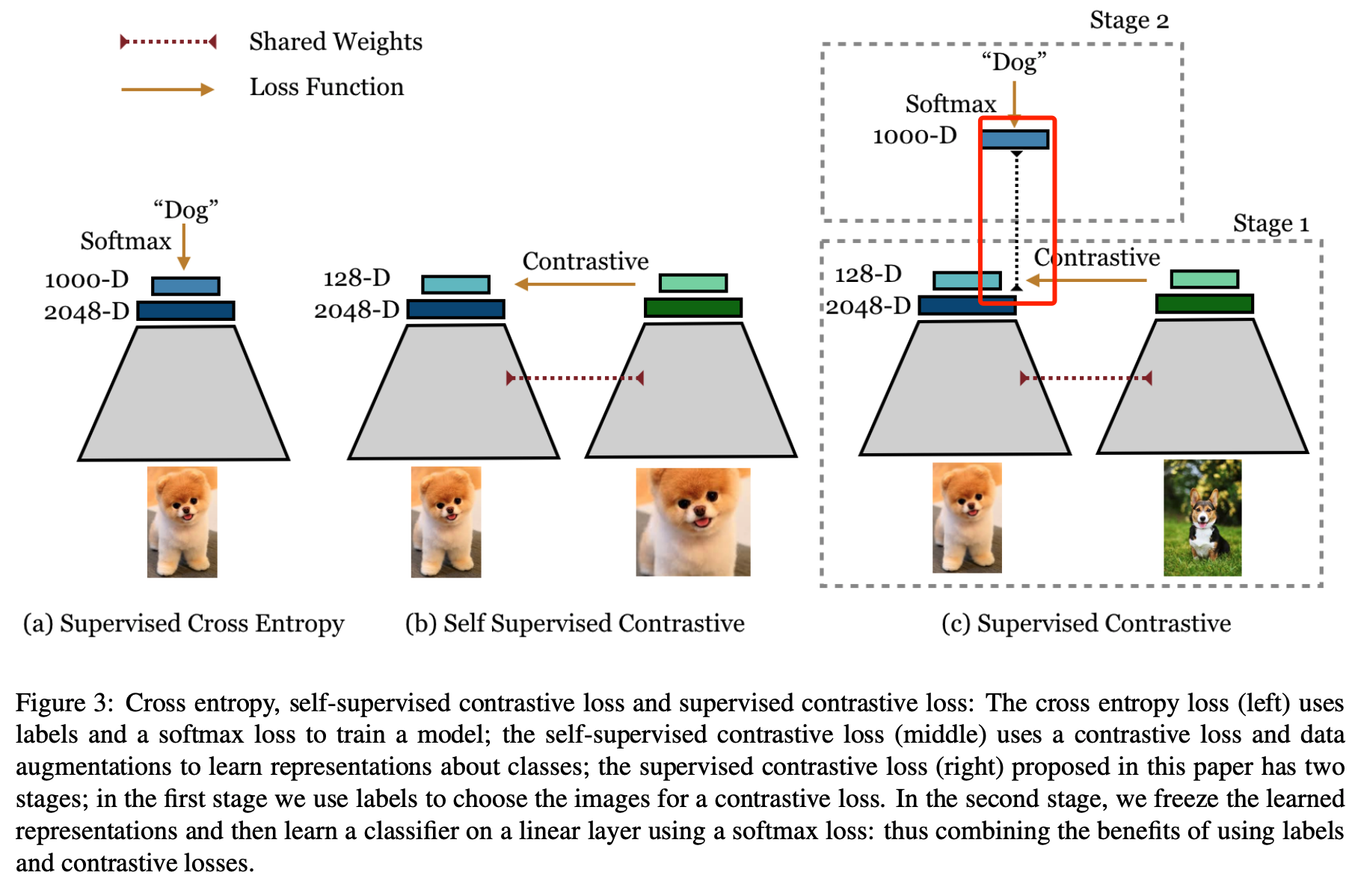
Supervised Contrastive Learning,Arxiv2004
- relation between triplet loss
- Analysis on ImageNet-C.
- batch size 8192 for ResNet-50 and batch size 2048 for ResNet-200;The LARS optimizer;RMSProp optimizer works best for training the linear classifier.
InfoMin: What Makes for Good Views for Contrastive Learning?Arxiv2005
- In this paper, we use empirical analysis to beer understand the importance of view selection, and argue that we should reduce the mutual information (MI) between views while keeping task-relevant information intact.
- Interesting experiment design about moving-mnist to validate the hypothesis.
Figure 5(Figure 5: 2048-dim of predictions from unsupervised pre-trained ResNet-50 on ImageNet-1K val set.) and the motivation of flatten?
Rethinking Image Mixture for Unsupervised Visual Representation Learning,Arxiv2003
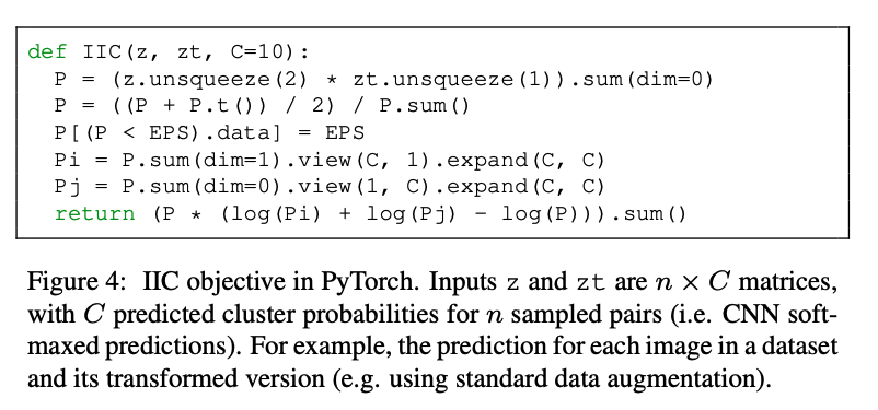
Invariant Information Clustering for Unsupervised Image Classification and Segmentation,ICCV19
train an image classifier or segmenter without any labelled data.
You have to know the class number \(C\) in advance.
for data augmentation, we repeat images within each batch r times; this means that multiple image pairs within a batch contain the same original image, each paired with a different transformation, which encourages greater distillation since there are more examples of which visual details to ignore (section 3.1)
Multi-head, similar to multi-head transformer: For increased robustness, each head is duplicated h = 5 times with a different random initialisation, and we call these concrete instantiations subheads. Each sub-head takes features from b and outputs a probability distribution for each batch element over the relevant number of clusters.
For IIC, the main and auxiliary heads are trained by maximising eq. (3) in alternate epochs.
PICA:Deep Semantic Clustering by Partition Confidence Maximisation,CVPR20
following IIC.
Deep Robust Clustering by Contrastive Learning,Arxiv2008
following PICA
Local Aggregation for Unsupervised Learning of Visual Embeddings
TODO
CLSA: Contrastive Learning with Stronger Augmentations,ICLR21 submission
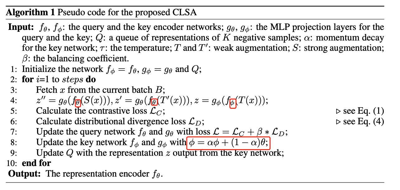
- Intuition: Instead of applying strongly augmented views to the contrastive loss, we propose to minimize the distribution divergence between the weakly and strongly augmented images over a representation bank to supervise the retrieval of stronger queries. This avoids an overoptimistic assumption that could overfit the strongly augmented queries containing distorted visual structures into the positive targets, while still being able to distinguish them from the negative samples by leveraging the distributions of weakly augmented counterparts. The learned representation will not only explore the novel patterns exposed by the stronger augmentations, but also inherits the knowledge about the relative similarities to the negative samples.
- Strong aug: In particular, to transform an image, we randomly select an augmentation from the above 14 types of transformations, and apply it to the image with a probability of 0.5. This process is repeated five times and that will strongly augment an image as the example shown in the right panel of Fig. 2.
- Typically, the experiment with a single strong augmentation for each training image takes roughly 70 hours to finish on 8 V100 GPUs.
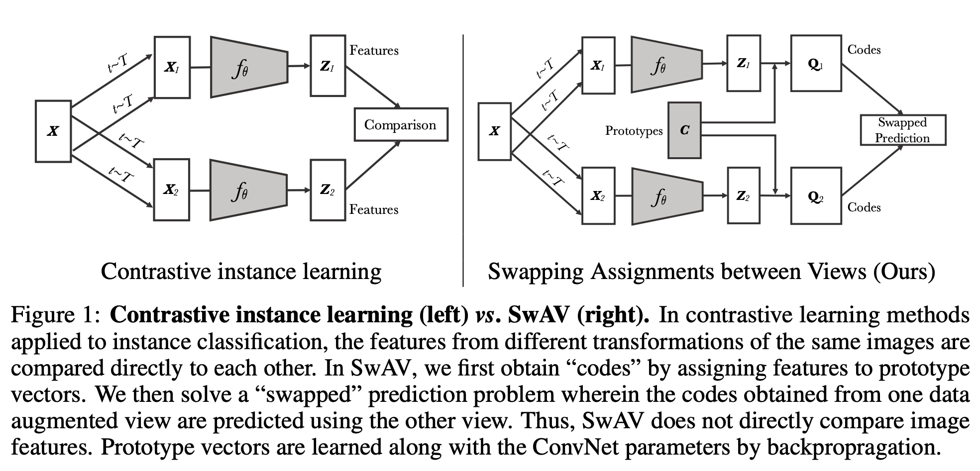
SwAV: Unsupervised Learning of Visual Features by Contrasting Cluster Assignments,Arxiv2006
- deep cluster->sela->Swav
- image x, feature z, code q, prototype c. \(q=z^{T}c\). B: batch size. K cluster size. C feature dimension from convnet.
- \[z \in C\times B, q \in B \times K , c \in C \times K\]
- An alternative to approximate the loss is to approximate the task—that is to relax the instance discrimination problem. For example, clustering-based methods discriminate between groups of images with similar features instead of individual images
- Swapped prediction problem. It seems that method can also work without swapping, it’s great if the author can ablate this.
- Check supp for pseudo-code.
- in Moco,SimCLR, ConSup, the negative sample is the image feature of another image. In clustering-based method, the negative sample is the typical feature of other cluster centers( a representative feature of other all negatives).
- Note that SwAV is the first self-supervised method to surpass ImageNet supervised features on these datasets, see Table 2.
- Also, Q is not binary(0 and 1 in Sela.ICLR20), Eq 2 is is soft cross-entropy(similar to label smoothing in mixup paper).
- \(tr(Q^{T} C^{T} Z)\), BxK, KxC, CxB(trace writing here is coherent to the inner product writing in SeLa) feature z is projected to the unit sphere by L2 normalization; prototype C is updated by gradient descent(Equation 2). Q is a probability matrix(transpotation polytope), as code q is code needed in cross entroy(equation 2), therefore, we need design a method to calculate q by matrix rescaling(better online)
- The online updating of Q is heavily borrowed from Self-labelling via simultaneous clustering and representation learning,ICLR20, why exp(CtZ/e) rather than Plamda in Sela in eq 5?
- multi-crop(large crop and small crop) is crucial, check Figure 3. As noted in prior works [10, 42], comparing random crops of an image plays a central role by capturing information in terms of relations between parts of a scene or an object.
- Interestingly, multi-crop seems to benefit more clustering-based methods than contrastive methods. We note that multi-crop does not improve the supervised model. see Fig 3.
- Supervised pretraining is too easy to saturate as model complexity increase. For SwAV, it can still take advantage of it. check Fig 4.
- We distribute the batches over 64 V100 16Gb GPUs, resulting in each GPU treating 64 instances.To help the very beginning of the optimization, we freeze the prototypes during the first epoch of training.Check more details in the supp. learning rate warm up. freeze prototype update in first epoch;
- Sharp point:Note that SwAV is more suitable for a multi-node distributed implementation compared to contrastive approaches SimCLR or MoCo. The latter methods require sharing the feature matrix across all GPUs at every batch which might become a bottleneck when distributing across many GPUs. On the contrary, SwAV requires sharing only matrix normalization statistics (sum of rows and columns) during the Sinkhorn algorithm.
- Number of prototypes is 8k, check C.1
Sela:Self-labelling via simultaneous clustering and representation learning,ICLR20
https://colab.research.google.com/drive/1F-FpHTVqurHN7OHIEb5Xld9T0Iv_RLDP
- Extension based on deep clustering.
- However, in the fully unsupervised case, it leads to a degenerate solution: eq. (1) is trivially minimized by assigning all data points to a single (arbitrary) label.
- Why Equation (5),Frobenius dot-product. mapping <kxN,kxN> to 1-dim. similar to inner product.
- optimization deduction, from Eq 7 to Eq 8?
- Why can be related to OT?
- P is log probability, after that, send them into sink-horn.
- Then, we compare our results to the state of the art in self-supervised representation learning, where we find that our method is the best among clustering-based techniques and overall state-of-the-art or at least highly competitive in many benchmarks.
- Following Xu Ji,2008, adopt a multi-head setting, similar to multi-task learninng. check 3.5
- Step 1 amounts to standard CE training, which we run for a fixed number of epochs. Step 2 can be interleaved at any point in the optimization; to amortize its cost, we run it at most once per epoch, and usually less, with a schedule described and validated below.
- Experimental analysis is interesting.
- By virtue of the method, the resulting self-labels can be used to quickly learn features for new architectures using simple cross-entropy training.
Labelling unlabelled videos from scratch with multi-modal self-supervision,Arxiv2006
A large part of the current success of deep learning lies in the effectiveness of data – more precisely: labelled data. Yet, labelling a dataset with human annotation continues to carry high costs, especially for videos. While in the image domain, recent methods have allowed to generate meaningful (pseudo-) labels for unlabelled datasets without supervision, this development is missing for the video domain where learning feature representations is the current focus. In this work, we a) show that unsupervised labelling of a video dataset does not come for free from strong feature encoders and b) propose a novel clustering method that allows pseudo-labelling of a video dataset without any human annotations, by leveraging the natural correspondence between the audio and visual modalities. An extensive analysis shows that the resulting clusters have high semantic overlap to ground truth human labels. We further introduce the first benchmarking results on unsupervised labelling of common video datasets Kinetics, Kinetics-Sound, VGG-Sound and AVE.
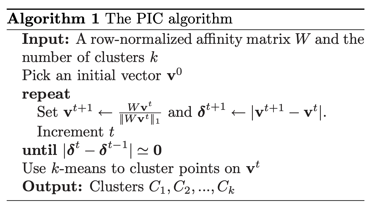
Power Iteration Clustering,ICML10
AND: Unsupervised Deep Learning by Neighbourhood Discovery,ICML19
- Without an extra classifier learning post-process involved, kNN reflects directly the discriminative capability of the learned feature representations.
- Dataset: CIFAR,SVHN,ImageNet,CUB200,Dogs.
Deep Clustering for Unsupervised Learning of Visual Features,ECCV18
Background: Despite the primeval success of clustering approaches in image classification, very few works [21,22] have been proposed to adapt them to the end-to-end training of convnets, and never at scale. An issue is that clustering methods have been primarily designed for linear models on top of fixed features, and they scarcely work if the features have to be learned simultaneously. For example, learning a convnet with k-means would lead to a trivial solution where the features are zeroed, and the clusters are collapsed into a single entity.
Note that running k-means takes a third of the time because a forward pass on the full dataset is needed. One could reassign the clusters every n epochs, but we found out that our setup on ImageNet (updating the clustering every epoch) was nearly optimal.
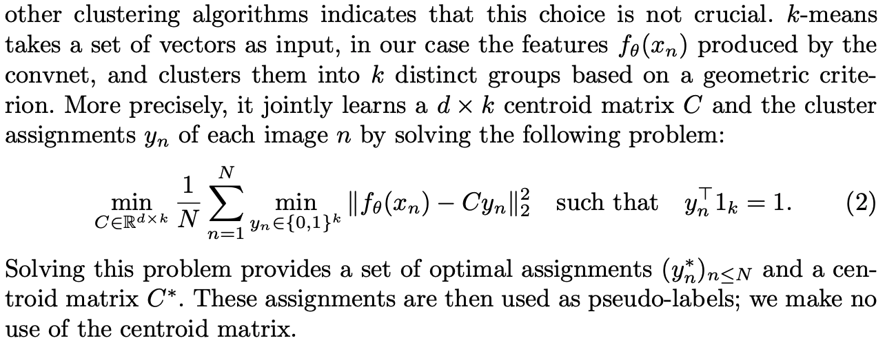
- C is dxk matrix, denoting the cenntriod of k centers with dimenstion d. even though K-means is non-parametric clustering. C can be implicitly obtained when convergent.
- Two stage optimization like ADMM. 1). update the parameters of the backbone by predicting these pseudo-labels. 2).update the dxk matrix(centriod feature/clustering center) by the new feature of overall dataset. This type of alternating procedure is prone to trivial solutions. Two tricky ways are introduced to avoid trival solutions.
- Interesting analysis in the experimental part.
- BTW, the order in the matrix is not important, you can even shuffle it, it’s not order-sensitive.
Memory-augmented Dense Predictive Coding for Video Representation Learning,ECCV20
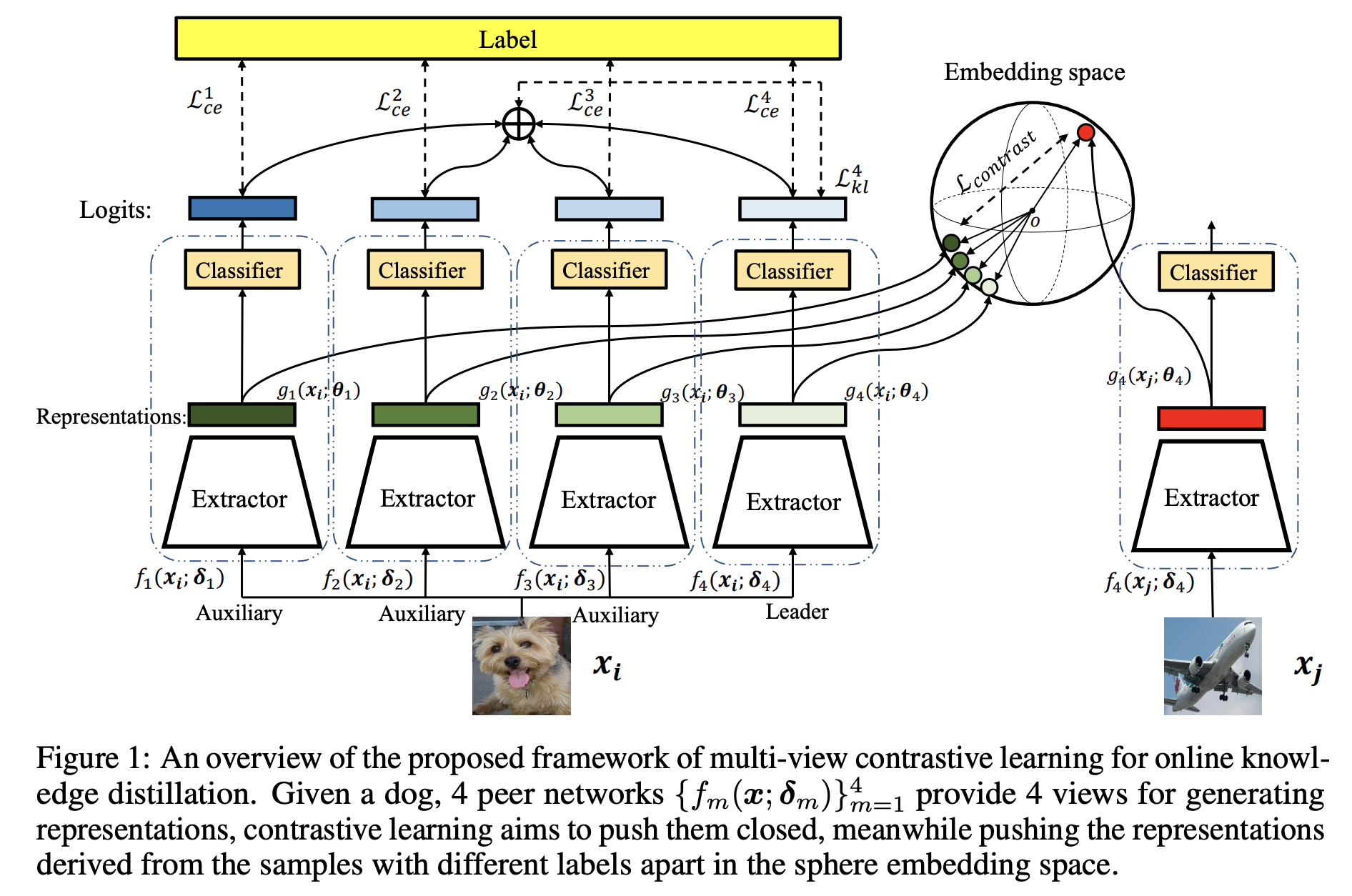
Multi-view Contrastive Learning for Online Knowledge Distillation,Arxiv2006
S4L: Self-Supervised Semi-Supervised Learning,ICCV19
- S4L-Rotation: a four-class cross-entropy loss
- S4L-examplar: similar to contrastive learning.
- baseline setting, virual adverersial training, conditional entropy mminimization(EntMin), Pseudo-label.
- Pseudo-label is very similar to self-training, while authentic self-traning utilizes the augmentation!
ClusterFit: Improving Generalization of Visual Representations,CVPR20
PIRL: Self-Supervised Learning of Pretext-Invariant Representations,CVPR20
Only consider jigsaw. In this work, we adopt the existing Jigsaw pretext task in a way that encourages the image representations to be invariant to the image patch perturbation.
Learning To Classify Images Without Labels
Online Deep Clustering for Unsupervised Representation Learning,CVPR20
Unsupervised Pre-Training of Image Features on Non-Curated Data,ICCV19
same author of deepcluster.
based on non-curated dataset YFCC100M.
Self-Supervised Learning of Video-Induced Visual Invariances,CVPR20
The proposed unsupervised models (VIVIEx(4) / VIVI-Ex(4)-Big) trained on raw Youtube8M videos and variants co-trained with 10%/100% labeled ImageNet data (VIVI-Ex(4)-Co(10%) / VIVI-Ex(4)-Co(100%)), outperform the corresponding unsupervised (Ex-ImageNet), semi-supervised (Semi-Ex-10%) and fully supervised (Sup100%, Sup-Rot-100%) baselines by a large margin.
shot supervision use augmentation as supervison.
video supervison use binary order prediction(forward or backward).
Self-supervised learning for video correspondence
Learning Correspondence from the Cycle-consistency of Time,
Self-supervised Learning for Video Correspondence Flow,BMVC19
MAST: A Memory-Augmented Self-Supervised Tracker,CVPR20
Application
Landmarks: Unsupervised Discovery of Object Landmarks via Contrastive Learning